Auto-tuning of a PID controller

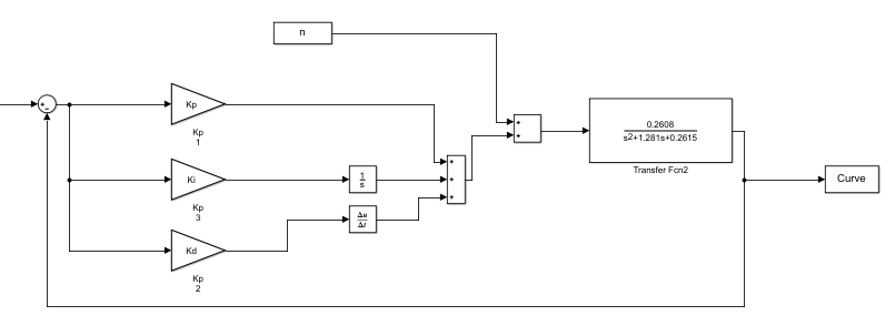
A proportional-integral-derivative controller (PID), is a system that allows to regulate the error of a result by means of feedback, with the objective of assimilating a reference value. The PID control consists of three parameters that define its behavior: the proportional value (K_p), the integral value (K_i) and the derivative value (K_d), coexisting as:

G_c = K_p + K_i/s + K_ds
The action of obtaining the values of the constants K_p, K_i and K_d is called tuning. There are several methods to tune a system, including Ziegler-Nichols (maximum gain method) and Cohen-Coon. These methods, are sometimes considered as tedious and imprecise, that’s why in this project, we are looking to optimize.

Problematic

To exploit the performance of a PID controller, we will explore the results obtained when self tuned and modeled as a stochastic sequential decision problem.

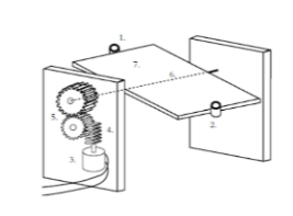
In Fig.1, we identify a system that needs to control its position, this system was analysed and roughly approximated to the following transfer function:
G_c = 0.2608/(s² + 1.281s + 0.2615)
this approximation is useful for simulations. Now, we can naively simulate the control of the system and stimulate it to obtain its reactions, the software used for this was Simulink from Matlab.

Solution

To solve, we will use a rollout algorithm.
The states x_k are composed by the gains K_i, K_p and K_d, and the curve resulting from their simulation. We can also define the system by its reference signal V_a, and a general terminal cost approximation (T_approx) denoted by:

T_approx= V_a

Our function to minimize is the expected value of the difference between the simulated curve and V_a at every state k (G_diff), seen as follows:

g_k(x_k, u_k) = E[|Curve_k − V_a|]

The control process will be defined by increasing one of this gains by a step whose distribution is denoted by U (0, 10). A second gain will be increased following a look-ahead policy, meaning that a mixure of two of the gains behavior of G_diff will be analyzed, as seen in:

J'_k = G_{diff k}

The G_diff will be a value constantly compared to find its optimal magnitude, if it’s a minimum value, we approve the path of gain increment so far, if G_diff didn’t improve, that gain increment will be discarded, being u_k and x_k+1 = f (x_k, u_k) defined.


Algorithm 1: Approximate method
Result: Gdiff, Ki, Kp, Kd

Ki, Kp, Kd, Va, Tapprox;

	While Tapprox > Gdiff do
		Increment gains sequentially, simulate and obtain Gdiffk;
		if Gdiffk < min(Gdif f ) then
			Update gains
		else
			Discard gains
		end
	end

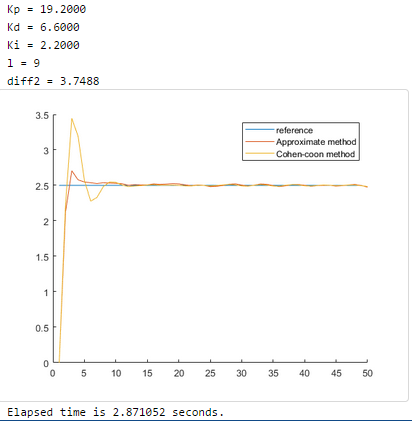
Results

This program takes an average of 5.56 seconds to find results for the PID controller. This is due to the fact that it needs more simulations for the look-ahead method. In the Fig. 3 we can see the results of one of the experiences. Here we note a better performance than the classic method of Cohen-coon.

Fig.3 - Solution for the PID parameters.

Implementation

MATLAB